Mplus is a statistical modeling program that provides researchers with a flexible tool to analyze their data. Mplus offers researchers a wide choice of models, estimators, and algorithms in a program that has an easy-to-use interface and graphical displays of data and analysis results. Mplus allows the analysis of both cross-sectional and longitudinal data, single-level and multilevel data, data that come from different populations with either observed or unobserved heterogeneity, and data that contain missing values. Analyses can be carried out for observed variables that are continuous, censored, binary, ordered categorical (ordinal), unordered categorical (nominal), counts, or combinations of these variable types. In addition, Mplus has extensive capabilities for Monte Carlo simulation studies, where data can be generated and analyzed according to most of the models included in the program.
The Mplus modeling framework draws on the unifying theme of latent variables. The generality of the Mplus modeling framework comes from the unique use of both continuous and categorical latent variables. Continuous latent variables are used to represent factors corresponding to unobserved constructs, random effects corresponding to individual differences in development, random effects corresponding to variation in coefficients across groups in hierarchical data, frailties corresponding to unobserved heterogeneity in survival time, liabilities corresponding to genetic susceptibility to disease, and latent response variable values corresponding to missing data. Categorical latent variables are used to represent latent classes corresponding to homogeneous groups of individuals, latent trajectory classes corresponding to types of development in unobserved populations, mixture components corresponding to finite mixtures of unobserved populations, and latent response variable categories corresponding to missing data.
THE Mplus MODELING FRAMEWORK
The purpose of modeling data is to describe the structure of data in a simple way so that it is understandable and interpretable. Essentially, the modeling of data amounts to specifying a set of relationships between variables. The figure below shows the types of relationships that can be modeled in Mplus. The rectangles represent observed variables. Observed variables can be outcome variables or background variables. Background variables are referred to as x; continuous and censored outcome variables are referred to as y; and binary, ordered categorical (ordinal), unordered categorical (nominal), and count outcome variables are referred to as u. The circles represent latent variables. Both continuous and categorical latent variables are allowed. Continuous latent variables are referred to as f. Categorical latent variables are referred to as c.
The arrows in the figure represent regression relationships between variables. Regressions relationships that are allowed but not specifically shown in the figure include regressions among observed outcome variables, among continuous latent variables, and among categorical latent variables. For continuous outcome variables, linear regression models are used. For censored outcome variables, censored (tobit) regression models are used, with or without inflation at the censoring point. For binary and ordered categorical outcomes, probit or logistic regressions models are used. For unordered categorical outcomes, multinomial logistic regression models are used. For count outcomes, Poisson and negative binomial regression models are used, with or without inflation at the zero point.
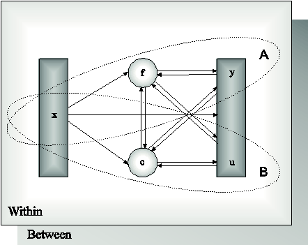
Models in Mplus can include continuous latent variables, categorical latent variables, or a combination of continuous and categorical latent variables. In the figure above, Ellipse A describes models with only continuous latent variables. Ellipse B describes models with only categorical latent variables. The full modeling framework describes models with a combination of continuous and categorical latent variables. The Within and Between parts of the figure above indicate that multilevel models that describe individual-level (within) and cluster-level (between) variation can be estimated using Mplus.
MODELING WITH CONTINUOUS LATENT VARIABLES
Ellipse A describes models with only continuous latent variables. Following are models in Ellipse A that can be estimated using Mplus:
· Regression analysis
· Path analysis
· Exploratory factor analysis
· Confirmatory factor analysis
· Item response theory modeling
· Structural equation modeling
· Growth modeling
· Discrete-time survival analysis
· Continuous-time survival analysis
· Time series analysis
Observed outcome variables can be continuous, censored, binary, ordered categorical (ordinal), unordered categorical (nominal), counts, or combinations of these variable types.
Special features available with the above models for all observed outcome variables types are:
· Single or multiple group analysis
· Missing data under MCAR, MAR, and NMAR and with multiple imputation
· Complex survey data features including stratification, clustering, unequal probabilities of selection (sampling weights), subpopulation analysis, replicate weights, and finite population correction
· Latent variable interactions and non-linear factor analysis using maximum likelihood
· Random slopes
· Individually-varying times of observations
· Linear and non-linear parameter constraints
· Indirect effects including specific paths
· Maximum likelihood estimation for all outcomes types
· Bootstrap standard errors and confidence intervals
· Wald chi-square test of parameter equalities
· Factor scores and plausible values for latent variables
MODELING WITH CATEGORICAL LATENT VARIABLES
Ellipse B describes models with only categorical latent variables. Following are models in Ellipse B that can be estimated using Mplus:
· Regression mixture modeling
· Path analysis mixture modeling
· Latent class analysis
· Latent class analysis with covariates and direct effects
· Confirmatory latent class analysis
· Latent class analysis with multiple categorical latent variables
· Loglinear modeling
· Non-parametric modeling of latent variable distributions
· Multiple group analysis
· Finite mixture modeling
· Complier Average Causal Effect (CACE) modeling
· Latent transition analysis and hidden Markov modeling including mixtures and covariates
· Latent class growth analysis
· Discrete-time survival mixture analysis
· Continuous-time survival mixture analysis
Observed outcome variables can be continuous, censored, binary, ordered categorical (ordinal), unordered categorical (nominal), counts, or combinations of these variable types. Most of the special features listed above are available for models with categorical latent variables. The following special features are also available.
· Analysis with between-level categorical latent variables
· Tests to identify possible covariates not included in the analysis that influence the categorical latent variables
· Tests of equality of means across latent classes on variables not included in the analysis
· Plausible values for latent classes
MODELING WITH BOTH CONTINUOUS AND CATEGORICAL LATENT VARIABLES
The full modeling framework includes models with a combination of continuous and categorical latent variables. Observed outcome variables can be continuous, censored, binary, ordered categorical (ordinal), unordered categorical (nominal), counts, or combinations of these variable types. Most of the special features listed above are available for models with both continuous and categorical latent variables. Following are models in the full modeling framework that can be estimated using Mplus:
· Latent class analysis with random effects
· Factor mixture modeling
· Structural equation mixture modeling
· Growth mixture modeling with latent trajectory classes
· Discrete-time survival mixture analysis
· Continuous-time survival mixture analysis
Most of the special features listed above are available for models with both continuous and categorical latent variables. The following special features are also available.
· Analysis with between-level categorical latent variables
· Tests to identify possible covariates not included in the analysis that influence the categorical latent variables
· Tests of equality of means across latent classes on variables not included in the analysis
MODELING WITH COMPLEX SURVEY DATA
There are two approaches to the analysis of complex survey data in Mplus. One approach is to compute standard errors and a chi-square test of model fit taking into account stratification, non-independence of observations due to cluster sampling, and/or unequal probability of selection. Subpopulation analysis, replicate weights, and finite population correction are also available. With sampling weights, parameters are estimated by maximizing a weighted loglikelihood function. Standard error computations use a sandwich estimator. For this approach, observed outcome variables can be continuous, censored, binary, ordered categorical (ordinal), unordered categorical (nominal), counts, or combinations of these variable types.
A second approach is to specify a model for each level of the multilevel data thereby modeling the non-independence of observations due to cluster sampling. This is commonly referred to as multilevel modeling. The use of sampling weights in the estimation of parameters, standard errors, and the chi-square test of model fit is allowed. Both individual-level and cluster-level weights can be used. With sampling weights, parameters are estimated by maximizing a weighted loglikelihood function. Standard error computations use a sandwich estimator. For this approach, observed outcome variables can be continuous, censored, binary, ordered categorical (ordinal), unordered categorical (nominal), counts, or combinations of these variable types.
The multilevel extension of the full modeling framework allows random intercepts and random slopes that vary across clusters in hierarchical data. Random slopes include the special case of random factor loadings. These random effects can be specified for any of the relationships of the full Mplus model for both independent and dependent variables and both observed and latent variables. Random effects representing across-cluster variation in intercepts and slopes or individual differences in growth can be combined with factors measured by multiple indicators on both the individual and cluster levels. In line with SEM, regressions among random effects, among factors, and between random effects and factors are allowed.
The two approaches described above can be combined. In addition to specifying a model for each level of the multilevel data thereby modeling the non-independence of observations due to cluster sampling, standard errors and a chi-square test of model fit are computed taking into account stratification, non-independence of observations due to cluster sampling, and/or unequal probability of selection. When there is clustering due to both primary and secondary sampling stages, the standard errors and chi-square test of model fit are computed taking into account the clustering due to the primary sampling stage and clustering due to the secondary sampling stage is modeled.
Most of the special features listed above are available for modeling of complex survey data.
MODELING WITH MISSING DATA
Mplus has several options for the estimation of models with missing data. Mplus provides maximum likelihood estimation under MCAR (missing completely at random), MAR (missing at random), and NMAR (not missing at random) for continuous, censored, binary, ordered categorical (ordinal), unordered categorical (nominal), counts, or combinations of these variable types (Little & Rubin, 2002). MAR means that missingness can be a function of observed covariates and observed outcomes. For censored and categorical outcomes using weighted least squares estimation, missingness is allowed to be a function of the observed covariates but not the observed outcomes (Asparouhov & Muthén, 2010a). When there are no covariates in the model, this is analogous to pairwise present analysis. Non-ignorable missing data (NMAR) modeling is possible using maximum likelihood estimation where categorical outcomes are indicators of missingness and where missingness can be predicted by continuous and categorical latent variables (Muthén, Jo, & Brown, 2003; Muthén et al., 2011).
In all models, missingness is not allowed for the observed covariates because they are not part of the model. The model is estimated conditional on the covariates and no distributional assumptions are made about the covariates. Covariate missingness can be modeled if the covariates are brought into the model and distributional assumptions such as normality are made about them. With missing data, the standard errors for the parameter estimates are computed using the observed information matrix (Kenward & Molenberghs, 1998). Bootstrap standard errors and confidence intervals are also available with missing data.
Mplus provides multiple imputation of missing data using Bayesian analysis (Rubin, 1987; Schafer, 1997). Both the unrestricted H1 model and a restricted H0 model can be used for imputation. Multiple data sets generated using multiple imputation can be analyzed using a special feature of Mplus. Parameter estimates are averaged over the set of analyses, and standard errors are computed using the average of the standard errors over the set of analyses and the between analysis parameter estimate variation (Rubin, 1987; Schafer, 1997). A chi-square test of overall model fit is provided (Asparouhov & Muthén, 2008c; Enders, 2010).
ESTIMATORS AND ALGORITHMS
Mplus provides both Bayesian and frequentist inference. Bayesian analysis uses Markov chain Monte Carlo (MCMC) algorithms. Posterior distributions can be monitored by trace and autocorrelation plots. Convergence can be monitored by the Gelman-Rubin potential scaling reduction using parallel computing in multiple MCMC chains. Posterior predictive checks are provided.
Frequentist analysis uses maximum likelihood and weighted least squares estimators. Mplus provides maximum likelihood estimation for all models. With censored and categorical outcomes, an alternative weighted least squares estimator is also available. For all types of outcomes, robust estimation of standard errors and robust chi-square tests of model fit are provided. These procedures take into account non-normality of outcomes and non-independence of observations due to cluster sampling. Robust standard errors are computed using the sandwich estimator. Robust chi-square tests of model fit are computed using mean and mean and variance adjustments as well as a likelihood-based approach. Bootstrap standard errors are available for most models. The optimization algorithms use one or a combination of the following: Quasi-Newton, Fisher scoring, Newton-Raphson, and the Expectation Maximization (EM) algorithm (Dempster et al., 1977). Linear and non-linear parameter constraints are allowed. With maximum likelihood estimation and categorical outcomes, models with continuous latent variables and missing data for dependent variables require numerical integration in the computations. The numerical integration is carried out with or without adaptive quadrature in combination with rectangular integration, Gauss-Hermite integration, or Monte Carlo integration.
MONTE CARLO SIMULATION CAPABILITIES
Mplus has extensive Monte Carlo facilities both for data generation and data analysis. Several types of data can be generated: simple random samples, clustered (multilevel) data, missing data, discrete- and continuous-time survival data, and data from populations that are observed (multiple groups) or unobserved (latent classes). Data generation models can include random effects and interactions between continuous latent variables and between categorical latent variables. Outcome variables can be generated as continuous, censored, binary, ordered categorical (ordinal), unordered categorical (nominal), counts, or combinations of these variable types. In addition, two-part (semicontinuous) variables and time-to-event variables can be generated. Independent variables can be generated as binary or continuous. All or some of the Monte Carlo generated data sets can be saved.
The analysis model can be different from the data generation model. For example, variables can be generated as categorical and analyzed as continuous or generated as a three-class model and analyzed as a two-class model. In some situations, a special external Monte Carlo feature is needed to generate data by one model and analyze it by a different model. For example, variables can be generated using a clustered design and analyzed ignoring the clustering. Data generated outside of Mplus can also be analyzed using this special external Monte Carlo feature.
Other special Monte Carlo features include saving parameter estimates from the analysis of real data to be used as population and/or coverage values for data generation in a Monte Carlo simulation study. In addition, analysis results from each replication of a Monte Carlo simulation study can be saved in an external file.
GRAPHICS
Mplus includes a dialog-based, post-processing graphics module that provides graphical displays of observed data and analysis results including outliers and influential observations.
These graphical displays can be viewed after the Mplus analysis is completed. They include histograms, scatterplots, plots of individual observed and estimated values, plots of sample and estimated means and proportions/probabilities, plots of estimated probabilities for a categorical latent variable as a function of its covariates, plots of item characteristic curves and information curves, plots of survival and hazard curves, plots of missing data statistics, plots of user-specified functions, and plots related to Bayesian estimation. These are available for the total sample, by group, by class, and adjusted for covariates. The graphical displays can be edited and exported as a DIB, EMF, or JPEG file. In addition, the data for each graphical display can be saved in an external file for use by another graphics program.
DIAGRAMMER
The Diagrammer can be used to draw an input diagram, to automatically create an output diagram, and to automatically create a diagram using an Mplus input without an analysis or data. To draw an input diagram, the Diagrammer is accessed through the Open Diagrammer menu option of the Diagram menu in the Mplus Editor. The Diagrammer uses a set of drawing tools and pop-up menus to draw a diagram. When an input diagram is drawn, a partial input is created which can be edited before the analysis. To automatically create an output diagram, an input is created in the Mplus Editor. The output diagram is automatically created when the analysis is completed. This diagram can be edited and used in a new analysis. The Diagrammer can be used as a drawing tool by using an input without an analysis or data.
Conditional probabilities, including latent transition probabilities, for different values of a set of covariates can be computed using the LTA Calculator. It is accessed by choosing LTA calculator from the Mplus menu of the Mplus Editor.
LANGUAGE GENERATOR
Mplus includes a language generator to help users create Mplus input files. The language generator takes users through a series of screens that prompts them for information about their data and model. The language generator contains all of the Mplus commands except DEFINE, MODEL, PLOT, and MONTECARLO. Features added after Version 2 are not included in the language generator.
The Mplus User’s Guide has 20 chapters. Chapter 2 describes how to get started with Mplus. Chapters 3 through 13 contain examples of analyses that can be done using Mplus. Chapter 14 discusses special issues. Chapters 15 through 19 describe the Mplus language. Chapter 20 contains a summary of the Mplus language. Technical appendices that contain information on modeling, model estimation, model testing, numerical algorithms, and references to further technical information can be found at www.statmodel.com.
It is not necessary to read the entire User’s Guide before using the program. A user may go straight to Chapter 2 for an overview of Mplus and then to one of the example chapters.