CHAPTER 18
OUTPUT, SAVEDATA, AND PLOT COMMANDS
In this chapter, the OUTPUT, SAVEDATA, and PLOT commands are discussed. The OUTPUT command is used to request additional output beyond that included as the default. The SAVEDATA command is used to save the analysis data and/or a variety of model results in an ASCII file for future use. The PLOT command is used to request graphical displays of observed data and analysis results.
The OUTPUT command is used to request additional output not included as the default.
Following are the option settings for the OUTPUT command:
|
OUTPUT: |
|
|
|
|
|
|
|
|
SAMPSTAT; |
|
|
|
CROSSTABS; |
ALL |
|
|
CROSSTABS (ALL); |
|
|
|
CROSSTABS (COUNT); |
|
|
|
CROSSTABS (%ROW); |
|
|
|
CROSSTABS (%COLUMN); |
|
|
|
CROSSTABS (%TOTAL); |
|
|
|
STANDARDIZED; |
|
|
|
STDYX; |
|
|
|
STDY; |
|
|
|
STD; |
|
|
|
STANDARDIZED (CLUSTER); |
|
|
|
STDYX (CLUSTER); STDY (CLUSTER); STD (CLUSTER); RESIDUAL; RESIDUAL (CLUSTER); |
|
|
|
MODINDICES (minimum chi-square); MODINDICES (ALL); MODINDICES (ALL minimum chi-square); |
10
10 |
|
|
CINTERVAL; CINTERVAL (SYMMETRIC); CINTERVAL (BOOTSTRAP); CINTERVAL (BCBOOTSTRAP); CINTERVAL (EQTAIL); CINTERVAL (HPD); |
SYMMETRIC
EQTAIL |
|
|
SVALUES; |
|
|
|
NOCHISQUARE; |
|
|
|
NOSERROR; |
|
|
|
H1SE; |
|
|
|
H1TECH3; H1MODEL; H1MODEL (COVARIANCE); H1MODEL (SEQUENTIAL); |
COVARIANCE |
|
|
PATTERNS; |
|
|
|
FSCOEFFICIENT; |
|
|
|
FSDETERMINACY; FSCOMPARISON; |
|
|
|
BASEHAZARD; |
|
|
|
LOGRANK; ALIGNMENT; |
|
|
|
ENTROPY; |
|
|
|
TECH1; |
|
|
|
TECH2; |
|
|
|
TECH3; |
|
|
|
TECH4; TECH4 (CLUSTER); |
|
|
|
TECH5; |
|
|
|
TECH6; |
|
|
|
TECH7; |
|
|
|
TECH8; |
|
|
|
TECH9; |
|
|
|
TECH10; |
|
|
|
TECH11; |
|
|
|
TECH12; |
|
|
|
TECH13; TECH14; TECH15; TECH16; |
|
The OUTPUT command is not a required command. Note that commands can be shortened to four or more letters. Option settings can be referred to by either the complete word or the part of the word shown above in bold type.
The default output for all analyses includes a listing of the input setup, a summary of the analysis specifications, and a summary of the analysis results. Analysis results include a set of fit statistics, parameter estimates, standard errors of the parameter estimates, the ratio of each parameter estimate to its standard error, and a two-tailed p-value for the ratio. Analysis results for TYPE=EFA include eigenvalues for the sample correlation matrix, a set of fit statistics, estimated rotated factor loadings and correlations and their standard errors, estimated residual variances and their standard errors, the factor structure matrix, and factor determinacies. Output for TYPE=BASIC includes sample statistics for the analysis data set and other descriptive information appropriate for the particular analysis.
Following is a description of the information that is provided in the output as the default. Information about optional output is described in the next section. The output can be shown in a plain text or HTML format. The default is plain text.
The first information printed in the Mplus output is a restatement of the input file. The restatement of the input instructions is useful as a record of which input produced the results provided in the output. Following is the input file that produced the output that will be used in this chapter to illustrate most of the output features:
TITLE: example for the output chapter
DATA: FILE = output.dat;
VARIABLE: NAMES = y1-y4 x;
MODEL: f BY y1-y4;
f ON x;
OUTPUT: SAMPSTAT MODINDICES (0) STANDARDIZED
RESIDUAL TECH1 TECH2 TECH3 TECH4
TECH5 FSCOEF FSDET CINTERVAL PATTERNS;
SAVEDATA: FILE IS output.sav;
SAVE IS FSCORES;
SUMMARY OF ANALYSIS SPECIFICATIONS
A summary of the analysis specifications is printed in the output after the restatement of the input instructions. This is useful because it shows how the program has interpreted the input instructions and read the data. It is important to check that the number of observations is as expected. It is also important to read any warnings and error messages that have been generated by the program. These contain useful information for understanding and modifying the analysis.
Following is the summary of the analysis for the example output:
SUMMARY OF ANALYSIS
Number of groups 1
Number of observations 500
Number of dependent variables 4
Number of independent variables 1
Number of continuous latent variables 1
Observed dependent variables
Continuous
Y1 Y2 Y3 Y4
Observed independent variables
X
Continuous latent variables
F
Estimator ML
Information matrix EXPECTED
Maximum number of iterations 1000
Convergence criterion 0.500D-04
Maximum number of steepest descent iterations 20
Input data file(s)
output.dat
Input data format FREE
The third part of the output consists of a summary of the analysis results. Fit statistics, parameter estimates, and standard errors can be saved in an external data set by using the RESULTS option of the SAVEDATA command. Following is a description of what is included in the output.
Tests of model fit are printed first. For most analyses, these consist of the chi-square test statistic, degrees of freedom, and p-value for the analysis model; the chi-square test statistic, degrees of freedom, and p-value for the baseline model of uncorrelated dependent variables; CFI and TLI; the loglikelihood for the analysis model; the loglikelihood for the unrestricted model; the number of free parameters in the estimated model; AIC, BIC, and sample-size adjusted BIC; RMSEA; and SRMR.
MODEL FIT INFORMATION
Number of Free Parameters 13
Loglikelihood
H0 Value -3329.929
H1 Value -3326.522
Information Criteria
Akaike (AIC) 6685.858
Bayesian (BIC) 6740.648
Sample-Size Adjusted BIC 6699.385
(n* = (n + 2) / 24)
Chi-Square Test of Model Fit
Value 6.815
Degrees of Freedom 5
P-Value 0.2348
RMSEA (Root Mean Square Error Of Approximation)
Estimate 0.027
90 Percent C.I. 0.000 0.072
Probability RMSEA <= .05 0.755
CFI/TLI
CFI 0.999
TLI 0.997
Chi-Square Test of Model Fit for the Baseline Model
Value 1236.962
Degrees of Freedom 10
P-Value 0.0000
SRMR (Standardized Root Mean Square Residual)
Value 0.012
The results of the model estimation are printed after the tests of model fit. The first column of the output labeled Estimates contains the model estimated value for each parameter. The parameters are identified using the conventions of the MODEL command. For example, factor loadings are found in the BY statements. Other regression coefficients are found in the ON statements. Covariances and residual covariances are found in the WITH statements. Variances, residual variances, means, intercepts, and thresholds are found under these headings. The scale factors used in the estimation of models with categorical outcomes are found under the heading Scales.
The type of regression coefficient produced during model estimation is determined by the scale of the dependent variable and the estimator being used in the analysis. For continuous observed dependent variables and for continuous latent dependent variables, the regression coefficients produced for BY and ON statements for all estimators are linear regression coefficients. For censored observed dependent variables, the regression coefficients produced for BY and ON statements for all estimators are censored-normal regression coefficients. For the inflation part of censored observed dependent variables, the regression coefficients produced for BY and ON statements are logistic regression coefficients. For binary and ordered categorical observed dependent variables, the regression coefficients produced for BY and ON statements using a weighted least squares estimator such as WLSMV are probit regression coefficients. For binary and ordered categorical observed dependent variables, the regression coefficients produced for BY and ON statements using a maximum likelihood estimator are logistic regression coefficients using the default LINK=LOGIT and probit regression coefficients using LINK=PROBIT. Logistic regression for ordered categorical outcomes uses the proportional odds specification. For categorical latent dependent variables and unordered categorical observed dependent variables, the regression coefficients produced for ON statements are multinomial logistic regression coefficients. For count observed dependent variables and time-to-event variables in continuous-time survival analysis, the regression coefficients produced for BY and ON statements are loglinear regression coefficients. For the inflation part of count observed dependent variables, the regression coefficients produced for BY and ON statements are logistic regression coefficients.
MODEL RESULTS
Two-Tailed
Estimate S.E. Est./S.E. P-Value
F BY
Y1 1.000 0.000 999.000 999.000
Y2 0.907 0.046 19.908 0.000
Y3 0.921 0.045 20.509 0.000
Y4 0.949 0.046 20.480 0.000
F ON
X 0.606 0.049 12.445 0.000
Intercepts
Y1 0.132 0.051 2.608 0.009
Y2 0.118 0.049 2.393 0.017
Y3 0.061 0.048 1.268 0.205
Y4 0.076 0.050 1.529 0.126
Residual Variances
Y1 0.479 0.043 11.061 0.000
Y2 0.558 0.045 12.538 0.000
Y3 0.492 0.041 11.923 0.000
Y4 0.534 0.044 12.034 0.000
F 0.794 0.073 10.837 0.000
The second column of the output labeled S.E. contains the standard errors of the parameter estimates. The type of standard errors produced during model estimation is determined by the estimator that is used. The estimator being used is printed in the summary of the analysis. Each analysis type has a default estimator. For several analysis types, the default estimator can be changed using the ESTIMATOR option of the ANALYSIS command. A table of estimators that are available for each analysis type can be found in Chapter 16.
The third column of the output labeled Est./S.E. contains the value of the parameter estimate divided by the standard error (column 1 divided by column 2). This statistical test is an approximately normally distributed quantity (z-score) in large samples. The critical value for a two-tailed test at the .05 level is an absolute value greater than 1.96. The fourth column of the output labeled Two-Tailed P-Value gives the p-value for the z-score in the third column.
The value of 999 is printed when a value cannot be computed. This happens most often when there are negative variances or residual variances. A series of asterisks (*) is printed when the value to be printed is too large to fit in the space provided. This happens when variables are measured on a large scale. To reduce the risk of computational difficulties, it is recommended to keep variables on a scale such that their variances do not deviate too far from the range of one to ten. Variables can be rescaled using the DEFINE command.
The SAMPSTAT option is used to request sample statistics for the data being analyzed. For continuous variables, these include sample means, sample variances, sample covariances, and sample correlations. In addition to these, the following univariate descriptive statistics are available: sample size, mean, variance, skewness, kurtosis, minimum, maximum, percent with minimum, percent with maximum, percentiles, and the median. For binary and ordered categorical (ordinal) variables using weighted least squares estimation, the sample statistics include sample thresholds; sample tetrachoric, polychoric and polyserial correlations for models without covariates; and sample probit regression coefficients and sample probit residual correlations for models with covariates. In addition to these, univariate proportions and counts are available. The SAMPSTAT option is not available for censored variables using maximum likelihood estimation, unordered categorical (nominal) variables, count variables, binary and ordered categorical (ordinal) variables using maximum likelihood estimation, and time-to-event variables. The sample correlation and covariance matrices can be saved in an ASCII file using the SAMPLE option of the SAVEDATA command.
The CROSSTABS option is used to request bivariate frequency tables for pairs of binary, ordered categorical (ordinal), and/or unordered categorical (nominal) variables. Row, column, and total counts are given along with row, column, and total percentages for each category of the variable and the total counts. The CROSSTAB option has the following settings: ALL, COUNT, %ROW, %COLUMN, and %TOTAL. The default is ALL. These settings can be used to request specific information in the bivariate frequency table. For example,
CROSSTABS (COUNT %ROW);
provides a bivariate frequency table with count and row percentages.
The STANDARDIZED option is used to request standardized parameter estimates and their standard errors and R-square. Standard errors are computed using the Delta method. Both symmetric and non-symmetric confidence intervals for standardized parameter estimates are available using the CINTERVAL option of the OUTPUT command.
Three types of standardizations are provided as the default. The first type of standardization is shown under the heading StdYX in the output. StdYX uses the variances of the continuous latent variables as well as the variances of the background and outcome variables for standardization. The StdYX standardization is the one used in the linear regression of y on x,
bStdYX = b*SD(x)/SD(y),
where b is the unstandardized linear regression coefficient, SD(x) is the sample standard deviation of x, and SD(y) is the model estimated standard deviation of y. The standardized coefficient bStdYX is interpreted as the change in y in y standard deviation units for a standard deviation change in x.
The second type of standardization is shown under the heading StdY in the output. StdY uses the variances of the continuous latent variables as well as the variances of the outcome variables for standardization. The StdY standardization for the linear regression of y on x is
bStdY = b/SD(y).
StdY should be used for binary covariates because a standard deviation change of a binary variable is not meaningful. The standardized coefficient bStdY is interpreted as the change in y in y standard deviation units when x changes from zero to one.
In mediation modeling where y is regressed on the mediator m and m is regressed on x, the StdY coefficient for y on m is standardized by both the standard deviation of y and the standard deviation of m because m is a dependent variable in the regression of m on x. StdY is therefore equivalent to StdYX in this case.
The third type of standardization is shown under the heading Std in the output. Std uses the variances of the continuous latent variables for standardization.
Covariances are standardized using variances. Residual covariances are standardized using residual variances. This is the case for both latent and observed variables.
Options are available to request one or two of the standardizations. They are STDYX, STDY, and STD. To request only the standardization that uses the variances of the continuous latent variables as well as the variances of the background and outcome variables, specify:
STDYX;
To request both the standardization that uses the variances of the continuous latent variables as well as the variances of the background and outcome variables and the standardization that uses the variances of the continuous latent variables and the variances of the outcome variables, specify:
STDYX STDY;
For models with random effects defined using the | symbol in conjunction with ON and BY and for random variances, the STANDARDIZED option is available for TYPE=TWOLEVEL and ESTIMATOR=BAYES. When a model has random effects, each parameter is standardized for each cluster. The standardized values reported are the average of the standardized values across clusters for each parameter (Schuurman et al., 2016; Asparouhov, Hamaker, & Muthén, 2017). The CLUSTER setting of the STANDARDIZED option is used when a model has random effects to request that the standardized values for each cluster be printed in the output. Following is an example of how to specify the STANDARDIZED option using the CLUSTER setting:
STANDARDIZED (CLUSTER);
The STANDARDIZED option is not available for TYPE=RANDOM with maximum likelihood estimation or the CONSTRAINT option of the VARIABLE command. For the MUML estimator, STDY and standard errors for standardized estimates are not available.
Following is the output obtained when requesting STDYX:
STDYX Standardization
Two-Tailed
Estimates S.E. Est./S.E. P-Value
F BY
Y1 0.838 0.018 47.679 0.000
Y2 0.790 0.020 38.807 0.000
Y3 0.813 0.019 42.691 0.000
Y4 0.810 0.019 42.142 0.000
F ON
X 0.545 0.034 15.873 0.000
Intercepts
Y1 0.104 0.040 2.605 0.009
Y2 0.097 0.040 2.391 0.017
Y3 0.051 0.040 1.269 0.205
Y4 0.061 0.040 1.529 0.126
Residual Variances
Y1 0.298 0.029 10.106 0.000
Y2 0.375 0.032 11.657 0.000
Y3 0.339 0.031 10.964 0.000
Y4 0.345 0.031 11.078 0.000
F 0.703 0.037 18.822 0.000
where the first column of the output labeled Estimates contains the parameter estimate that has been standardized using the variances of the continuous latent variables as well as the variances of the background and outcome variables for standardization, the second column of the output labeled S.E. contains the standard error of the standardized parameter estimate, the third column of the output labeled Est./S.E. contains the value of the parameter estimate divided by the standard error (column 1 divided by column 2), and the fourth column of the output labeled Two-Tailed P-Value gives the p-value for the z-score in the third column. When standardized parameter estimates and standard errors are requested, an R-square value and its standard error are given for each observed and latent dependent variable in the model.
The RESIDUAL option is used to request residuals for the observed variables in the analysis. Residuals are computed for the model estimated means/intercepts/thresholds and the model estimated covariances/correlations/residual correlations. Residuals are computed as the difference between the value of the observed sample statistic and its model-estimated value. With missing data, the observed sample statistics are replaced by the estimated unrestricted model for the means/intercepts/thresholds and the covariances/correlations/residual correlations. Standardized and normalized residuals are available for continuous outcomes with TYPE=GENERAL and maximum likelihood estimation. Standardized residuals are computed as the difference between the value of the observed sample statistic and its model estimated value divided by the standard deviation of the difference between the value of the observed sample statistic and its model estimated value. Standardized residuals are approximate z-scores. Normalized residuals are computed as the difference between the value of the observed sample statistic and its model estimated value divided by the standard deviation of the value of the observed sample statistic. The RESIDUAL option is not available for TYPE=RANDOM with maximum likelihood estimation or the CONSTRAINT option of the VARIABLE command.
or models with random effects defined using the | symbol in conjunction with ON and BY and for random variances, the RESIDUAL option is available for TYPE=TWOLEVEL and ESTIMATOR=BAYES. The CLUSTER setting of the RESIDUAL option is used when a model has random effects to request that residuals for each cluster be printed in the output. Following is an example of how to specify RESIDUAL option using the CLUSTER setting:
RESIDUAL (CLUSTER);
Following is an example of the residual output for a covariance matrix:
RESIDUAL OUTPUT
ESTIMATED MODEL AND RESIDUALS (OBSERVED - ESTIMATED)
Model Estimated Covariances/Correlations/Residual Correlations
Y1 Y2 Y3 Y4 X
________ ________ ________ ________ ________
Y1 1.608
Y2 1.024 1.487
Y3 1.041 0.944 1.451
Y4 1.072 0.972 0.987 1.551
X 0.553 0.501 0.509 0.524 0.912
Residuals for Covariances/Correlations/Residual Correlations
Y1 Y2 Y3 Y4 X
________ ________ ________ ________ ________
Y1 0.000
Y2 0.004 0.000
Y3 -0.014 0.013 0.000
Y4 -0.006 0.002 0.005 0.000
X 0.040 -0.048 -0.003 0.000 0.000
Standardized Residuals (z-scores) for Covariances/Correlations/
Residual Correlations
Y1 Y2 Y3 Y4 X
________ ________ ________ ________ ________
Y1 0.000
Y2 0.252 0.000
Y3 -1.241 0.819 0.000
Y4 -0.505 0.143 0.336 0.000
X 1.906 -2.284 -0.132 -0.003 0.000
Normalized Residuals for Covariances/Correlations/Residual
Correlations
Y1 Y2 Y3 Y4 X
________ ________ ________ ________ ________
Y1 0.000
Y2 0.043 0.000
Y3 -0.165 0.171 0.000
Y4 -0.073 0.029 0.061 0.00
X 0.664 -0.864 -0.049 -0.001 0.000
The MODINDICES option is used to request the following indices: modification indices, expected parameter change indices, and two types of standardized expected parameter change indices for all parameters in the model that are fixed or constrained to be equal to other parameters. Model modification indices are available for most models when observed dependent variables are continuous, binary, and ordered categorical (ordinal). The MODINDICES option is used with EFA to request modification indices and expected parameter change indices for the residual correlations. The MODINDICES option is not available for the MODEL CONSTRAINT command, ALGORITHM=INTEGRATION, TYPE=TWOLEVEL using the MUML estimator, the BOOTSTRAP option of the ANALYSIS command, and for models with more than one categorical latent variable.
When model modification indices are requested, they are provided as the default when the modification index for a parameter is greater than or equal to 10. The following statement requests modification indices greater than zero:
MODINDICES (0);
Model modification indices are provided for the matrices that are opened as part of the analysis. To request modification indices for all matrices, specify:
MODINDICES (ALL);
or
MODINDICES (ALL 0);
The first column of the output labeled M.I. contains the modification index for each parameter that is fixed or constrained to be equal to another parameter. A modification index gives the expected drop in chi-square if the parameter in question is freely estimated. The parameters are labeled using the conventions of the MODEL command. For example, factor loadings are found in the BY statements. Other regression coefficients are found in the ON statements. Covariances and residual covariances are found in the WITH statements. Variances, residual variances, means, intercepts, and thresholds are found under these headings. The scale factors used in the estimation of models with categorical outcomes are found under the heading Scales.
MODEL MODIFICATION INDICES
Minimum M.I. value for printing the modification index 0.000
M.I. E.P.C. Std E.P.C. StdYX E.P.C.
WITH Statements
Y2 WITH Y1 0.066 0.010 0.010 0.019
Y3 WITH Y1 1.209 -0.042 -0.042 -0.086
Y3 WITH Y2 0.754 0.031 0.031 0.059
Y4 WITH Y1 0.226 -0.019 -0.019 -0.037
Y4 WITH Y2 0.021 0.005 0.005 0.010
Y4 WITH Y3 0.116 0.013 0.013 0.024
The second column of the output labeled E.P.C. contains the expected parameter change index for each parameter that is fixed or constrained to be equal to another parameter. An E.P.C. index provides the expected value of the parameter in question if it is freely estimated. The third and fourth columns of the output labeled Std E.P.C. and StdYX E.P.C. contain the two standardized expected parameter change indices. These indices are useful because the standardized values provide relative comparisons. The Std E.P.C. indices are standardized using the variances of the continuous latent variables. The StdYX E.P.C. indices are standardized using the variances of the continuous latent variables as well as the variances of the background and/or outcome variables.
The CINTERVAL option is used to request confidence intervals for frequentist model parameter estimates and credibility intervals for Bayesian model parameter estimates. Confidence intervals are also available for indirect effects and standardized indirect effects. The CINTERVAL option has three settings for frequentist estimation and two settings for Bayesian estimation.
The frequentist settings are SYMMETRIC, BOOTSTRAP, and BCBOOTSTRAP. SYMMETRIC is the default for frequentist estimation. SYMMETRIC produces 90%, 95% and 99% symmetric confidence intervals. BOOTSTRAP produces 90%, 95%, and 99% bootstrap confidence intervals. BCBOOTSTRAP produces 90%, 95%, and 99% bias-corrected bootstrap confidence intervals. The bootstrapped distribution of each parameter estimate is used to determine the bootstrap and bias-corrected bootstrap confidence intervals. These intervals take non-normality of the parameter estimate distribution into account. As a result, they are not necessarily symmetric around the parameter estimate.
The Bayesian settings are EQTAIL and HPD. EQTAIL is the default for Bayesian estimation. EQTAIL produces 90%, 95%, and 99% credibility intervals of the posterior distribution with equal tail percentages. HPD produces 90%, 95%, and 99% credibility intervals of the posterior distribution that give the highest posterior density (Gelman et al., 2004).
With frequentist estimation, only SYMMETRIC confidence intervals are available for standardized parameter estimates. With Bayesian estimation, both EQTAIL and HPD confidence intervals are available for standardized parameter estimates.
The following statement shows how to request bootstrap confidence intervals:
CINTERVAL (BOOTSTRAP);
In the output, the parameters are labeled using the conventions of the MODEL command. For example, factor loadings are found in the BY statements. Other regression coefficients are found in the ON statements. Covariances and residual covariances are found in the WITH statements. Variances, residual variances, means, intercepts, and thresholds will be found under these headings. The scale factors used in the estimation of models with categorical outcomes are found under the heading Scales. The CINTERVAL option is not available for TYPE=EFA.
The outputs for frequentist confidence intervals and Bayesian credibility intervals have the same format. Following is output showing symmetric frequentist confidence intervals:
CONFIDENCE INTERVALS OF MODEL RESULTS Lower .5% Lower 2.5% Lower 5% Estimate Upper 5% Upper 2.5% Upper .5% F BYY1 1.000 1.000 1.000 1.000 1.000 1.000 1.000Y2 0.790 0.818 0.832 0.907 0.982 0.996 1.024Y3 0.806 0.833 0.847 0.921 0.995 1.009 1.037Y4 0.829 0.858 0.872 0.949 1.025 1.039 1.068 F ONX 0.481 0.511 0.526 0.606 0.686 0.702 0.732 InterceptsY1 0.002 0.033 0.049 0.132 0.215 0.231 0.262Y2 -0.009 0.021 0.037 0.118 0.199 0.214 0.245Y3 -0.063 -0.033 -0.018 0.061 0.141 0.156 0.186Y4 -0.052 -0.022 -0.006 0.077 0.159 0.175 0.205 Residual VariancesY1 0.367 0.394 0.408 0.479 0.550 0.564 0.590Y2 0.443 0.471 0.485 0.558 0.631 0.645 0.673Y3 0.386 0.411 0.424 0.492 0.560 0.573 0.599Y4 0.420 0.447 0.461 0.534 0.607 0.621 0.649F 0.606 0.651 0.674 0.794 0.915 0.938 0.983
The fourth column of the output labeled Estimate contains the parameter estimates. The third and fifth columns of the output labeled Lower 5% and Upper 5%, respectively, contain the lower and upper bounds of the 90% confidence interval. The second and sixth columns of the output labeled Lower 2.5% and Upper 2.5%, respectively, contain the lower and upper bounds of the 95% confidence interval. The first and seventh columns of the output labeled Lower .5% and Upper .5%, respectively, contain the lower and upper bounds of the 99% confidence interval.
SVALUES
The SVALUES option is used to create input statements that contain parameter estimates from the analysis. These values are used as starting values in the input statements. The input statements can be used in a subsequent analysis in the MODEL or MODEL POPULATION commands. Not all input statements are reported, for example, input statements with the | symbol followed by ON, AT, or XWITH. For MODEL CONSTRAINT, input statements are created for only the parameters of the NEW option. Input statements are created as the default when a model does not converge. To request that these input statements be created, specify the following:
SVALUES;
The NOCHISQUARE option is used to request that the chi-square fit statistic not be computed. This reduces computational time when the model contains many observed variables. The chi-square fit statistic is computed as the default when available. To request that the chi-square fit statistic not be computed, specify the following:
NOCHISQUARE;
This option is not available for the MONTECARLO command unless missing data are generated.
The NOSERROR option is used to request that standard errors not be computed. This reduces computational time when the model contains many observed variables. To request that standard errors not be computed, specify the following:
NOSERROR;
This option is not available for the MONTECARLO command.
H1SE
The H1SE option is used with the ML, MLR, and MLF estimators to request standard errors for the unrestricted H1 model. It must be used in conjunction with TYPE=BASIC or the SAMPSTAT option of the OUTPUT command. It is not available for any other analysis type and it cannot be used in conjunction with the BOOTSTRAP option of the ANALYSIS command.
The H1TECH3 option is used to request estimated covariance and correlation matrices for the parameter estimates of the unrestricted H1 model. It is not available for any other analysis types, and it cannot be used in conjunction with the BOOTSTRAP option of the ANALYSIS command.
For TYPE=GENERAL and the DISTRIBUTION option of the ANALYSIS command, a chi-square test of model fit is available for testing the H0 model against an unrestricted model of means, variances, covariances, skew, and degrees of freedom using the H1MODEL option (Asparouhov & Muthén, 2015a). This test is not provided by default because it can be computationally demanding. The H1MODEL has two settings: COVARIANCE and SEQUENTIAL. The default is COVARIANCE. Following is an example of how to specify the SEQUENTIAL setting:
H1MODEL (SEQUENTIAL);
The PATTERNS option is used to request a summary of missing data patterns. The first part of the output shows the missing data patterns that occur in the data. In the example below, there are 13 patterns of missingness. In pattern 1, individuals are observed on y1, y2, y3, and y4. In pattern 7, individuals are observed on y1 and y4.
SUMMARY OF MISSING DATA PATTERNS
MISSING DATA PATTERNS (x = not missing)
1 2 3 4 5 6 7 8 9 10 11 12 13
Y1 x x x x x x x x
Y2 x x x x x x x Y3 x x x x x x x Y4 x x x x x xMISSING DATA PATTERN FREQUENCIES
Pattern Frequency Pattern Frequency Pattern Frequency
1 984 6 12 11 1
2 127 7 14 12 1
3 56 8 87 13 1
4 139 9 9
5 48 10 3
The second part of the output shows the frequency with which each pattern is observed in the data. For example, 984 individuals have pattern 1 whereas 14 have pattern 7.
The FSCOEFFICIENT option is used to request factor score coefficients and a factor score posterior covariance matrix. It is available only for TYPE=GENERAL and TYPE=COMPLEX with all continuous dependent variables. The factor score posterior covariance matrix is the variance/covariance matrix of the factor scores. Following is the information produced by the FSCOEFFICIENT option:
FACTOR SCORE INFORMATION (COMPLETE DATA)
FACTOR SCORE COEFFICIENTS
Y1 Y2 Y3 Y4 X
________ ________ ________ ________ ________
F 0.254 0.197 0.227 0.216 0.093
FACTOR SCORE POSTERIOR COVARIANCE MATRIX
F
________
F 0.122
The FSDETERMINACY option is used to request a factor score determinacy value for each factor in the model. It is available only for TYPE=EFA, TYPE=GENERAL, and TYPE=COMPLEX with all continuous dependent variables. The factor score determinacy is the correlation between the estimated and true factor scores. It ranges from zero to one and describes how well the factor is measured with one being
the best value. Following is the information produced by the FSDETERMINACY option:
FACTOR DETERMINACIES
F 0.945
The FSCOMPARISON option is used with ESTIMATOR=BAYES in conjunction with TYPE=TWOLEVEL to request a comparison of between-level estimated factor scores.
The BASEHAZARD option is used to request baseline hazard values for each time interval used in a continuous-time survival analysis. This option is available only with the SURVIVAL option. The baseline hazard values can be saved using the BASEHAZARD option of the SAVEDATA command.
With TYPE=MIXTURE, the LOGRANK option is used to request the logrank test also known as the Mantel-Cox test (Mantel, 1966). This test compares the survival distributions between pairs of classes for both continuous-time and discrete-time survival models. It is a nonparametric test for right-censored data. For discrete-time survival models, the DSURVIVAL option of the VARIABLE command must be used to identify the discrete-time survival variables.
The ALIGNMENT option is used with the ALIGNMENT option of the ANALYSIS command to obtain detailed measurement invariance test results for all items and factor mean comparisons for all pairs of groups.
The ENTROPY option is used in conjunction with TYPE=MIXTURE to request the entropy contribution for each latent class indicator. This information is useful for understanding each indicator’s importance in distinguishing among the latent classes. This variable-specific entropy is described in Asparouhov and Muthén (2014d).
The TECH1 option is used to request the arrays containing parameter specifications and starting values for all free parameters in the model. The number assigned to the parameter in the parameter specification matrices is the number used to refer to the parameter in error messages regarding non-identification and other issues. When saving analysis results, the parameters are saved in the order used in the parameter specification matrices. The starting values are shown in the starting value matrices. The TECH1 option is not available for TYPE=EFA.
TECHNICAL 1 OUTPUT
PARAMETER SPECIFICATION
NU
Y1 Y2 Y3 Y4 X
________ ________ ________ ________ ________
1 2 3 4 0
LAMBDA
F X
________ ________
Y1 0 0
Y2 5 0
Y3 6 0
Y4 7 0
X 0 0
THETA
Y1 Y2 Y3 Y4 X
________ ________ ________ ________ ________
Y1 8
Y2 0 9
Y3 0 0 10
Y4 0 0 0 11
X 0 0 0 0 0
ALPHA
F X
________ ________
0 0
BETA F X ________ ________ F 0 12 X 0 0 PSI F X________ ________
F 13
X 0 0
STARTING VALUES
NU Y1 Y2 Y3 Y4 X ________ ________ ________ ________ ________ 0.104 0.092 0.035 0.050 0.000 LAMBDA F X________ ________
Y1 1.000 0.000
Y2 1.000 0.000
Y3 1.000 0.000
Y4 1.000 0.000
X 0.000 1.000
THETA
Y1 Y2 Y3 Y4 X
________ ________ ________ ________ ________
Y1 0.806
Y2 0.000 0.745
Y3 0.000 0.000 0.727
Y4 0.000 0.000 0.000 0.777
X 0.000 0.000 0.000 0.000 0.000
ALPHA
F X
________ ________ 0.000 -0.046 BETA F X ________ ________ F 0.000 0.000 X 0.000 0.000 PSI F X________ ________
F 0.050
X 0.000 0.912
The TECH2 option is used to request parameter derivatives. The TECH2 option is not available for TYPE=EFA and the CONSTRAINT option of the VARIABLE command unless TYPE=MIXTURE is used.
TECHNICAL 2 OUTPUT
DERIVATIVES
Derivatives With Respect to NU
Y1 Y2 Y3 Y4 X
________ ________ ________ ________ ________
0.000 0.000 0.000 0.000 0.000
Derivatives With Respect to LAMBDA
F X
________ ________
Y1 0.000 -0.084
Y2 0.000 0.086
Y3 0.000 0.006
Y4 0.000 0.000
X 0.000 -0.014
Derivatives With Respect to THETA
Y1 Y2 Y3 Y4 X
________ ________ ________ ________ ________
Y1 0.000
Y2 -0.014 0.000
Y3 0.058 -0.049 0.000
Y4 0.024 -0.008 -0.019 0.000
X 0.000 0.000 0.000 0.000 0.000
Derivatives With Respect to ALPHA
F X
________ ________
0.000 0.000
Derivatives With Respect to BETA
F X
________ ________
F 0.000 0.000
X 0.000 0.000
Derivatives With Respect to PSI
F X
________ ________
F 0.000
X 0.000 0.000
The TECH3 option is used to request estimated covariance and correlation matrices for the parameter estimates. The parameters are referred to using the numbers assigned to them in TECH1. The TECH3 covariance matrix can be saved using the TECH3 option of the SAVEDATA command. The TECH3 option is not available for ESTIMATOR=ULS, the BOOTSTRAP option of the ANALYSIS command, and TYPE=EFA.
The TECH4 option is used to request estimated means, covariances, and correlations for the latent variables in the model. In addition to the means, covariances, and correlations, standard errors and p-values are given. The TECH4 means and covariance matrix can be saved using the TECH4 option of the SAVEDATA command. The TECH4 option is not available for TYPE=RANDOM with maximum likelihood estimation, the CONSTRAINT option of the VARIABLE command, or TYPE=EFA.
For models with random effects defined using the | symbol in conjunction with ON and BY and for random variances, the TECH4 option is available for TYPE=TWOLEVEL and ESTIMATOR=BAYES. The CLUSTER setting of the TECH4 option is used when a model has random effects to request that estimated means, covariances, and correlations for each cluster be printed in the output. Following is an example of how to specify the TECH4 option using the CLUSTER setting:
TECH4 (CLUSTER);
TECH5
The TECH5 option is used to request the optimization history in estimating the model. The TECH5 option is not available for TYPE=EFA.
The TECH6 option is used to request the optimization history in estimating sample statistics for categorical observed dependent variables. TECH6 is produced when at least one outcome variable is categorical but not when all outcomes are binary unless there is an independent variable in the model.
The TECH7 option is used in conjunction with TYPE=MIXTURE to request sample statistics for each class using raw data weighted by the estimated posterior probabilities for each class.
The TECH8 option is used to request that the optimization history in estimating the model be printed in the output. TECH8 is printed to the screen during the computations as the default. TECH8 screen printing is useful for determining how long the analysis takes. TECH8 is available for TYPE=RANDOM, MIXTURE, TWOLEVEL and analyses where numerical integration is used.
The TECH9 option is used in conjunction with the MONTECARLO command, the MONTECARLO and IMPUTATION options of the DATA command, and the BOOTSTRAP option of the ANALYSIS command to request error messages related to convergence for each replication or bootstrap draw. These messages are suppressed if TECH9 is not specified.
The TECH10 option is used to request univariate, bivariate, and response pattern model fit information for the categorical dependent variables in the model. This includes observed and estimated (expected) frequencies and standardized residuals. TECH10 is available for TYPE=MIXTURE and categorical and count variables with maximum likelihood estimation.
The TECH11 option is used in conjunction with TYPE=MIXTURE to request the Lo-Mendell-Rubin likelihood ratio test of model fit (Lo, Mendell, & Rubin, 2001) that compares the estimated model with a model with one less class than the estimated model. The Lo-Mendell-Rubin approach has been criticized (Jeffries, 2003) although it is unclear to which extent the critique affects its use in practice. The p-value obtained represents the probability that the data have been generated by the model with one less class. A low p-value indicates that the model with one less class is rejected in favor of the estimated model. An adjustment to the test according to Lo-Mendell-Rubin is also given. The model with one less class is obtained by deleting the first class in the estimated model. Because of this, it is recommended when using starting values that they be chosen so that the last class is the largest class. In addition, it is recommended that model identifying restrictions not be included in the first class. TECH11 is available only for ESTIMATOR=MLR. The TECH11 option is not available for the MODEL CONSTRAINT command, the BOOTSTRAP option of the ANALYSIS command, training data, and for models with more than one categorical latent variable.
The TECH12 option is used in conjunction with TYPE=MIXTURE to request residuals for observed versus model estimated means, variances, covariances, univariate skewness, and univariate kurtosis. The observed values come from the total sample. The estimated values are computed as a mixture across the latent classes. The TECH12 option is not available for TYPE=RANDOM, the MONTECARLO command, the CONSTRAINT option of the VARIABLE command, and when there are no continuous dependent variables.
The TECH13 option is used in conjunction with TYPE=MIXTURE to request two-sided tests of model fit for univariate, bivariate, and multivariate skew and kurtosis (Mardia’s measure of multivariate kurtosis). Observed sample values are compared to model estimated values generated over 200 replications. Each p-value obtained represents the probability that the estimated model has generated the data. A high p-value indicates that the estimated model fits the data. TECH13 is available only when the LISTWISE option of the DATA command is set to ON. TECH13 is not available for TYPE=TWOLEVEL MIXTURE, ALGORITHM=INTEGRATION, the BOOTSTRAP option of the ANALYSIS command, the CONSTRAINT option of the VARIABLE command, and when there are no continuous dependent variables.
The TECH14 option is used in conjunction with TYPE=MIXTURE to request a parametric bootstrapped likelihood ratio test (McLachlan and Peel, 2000) that compares the estimated model to a model with one less class than the estimated model. The p-value obtained represents an approximation to the probability that the data have been generated by the model with one less class. A low p-value indicates that the model with one less class is rejected in favor of the estimated model. The model with one less class is obtained by deleting the first class in the estimated model. Because of this, it is recommended that model identifying restrictions not be included in the first class. In addition, it is recommended when using starting values that they be chosen so that the last class is the largest class. TECH14 is not available for TYPE=RANDOM unless ALGORITHM=INTEGRATION is used, the BOOTSTRAP option of the ANALYSIS command, training data, the CONSTRAINT option of the VARIABLE command, with sampling weights, and for models with more than one categorical latent variable.
Following is a description of the bootstrap method that is used in TECH14. Models are estimated for both the number of classes in the analysis model (k) and the number of classes in the analysis model minus one (k–1). The loglikelihood values from the k and k-1 class analyses are used to compute a likelihood ratio test statistic (-2 times the loglikelihood difference). Several data sets, referred to as bootstrap draws, are then generated using the parameter estimates from the k-1 class model. These data are analyzed for both the k and k-1 class models to obtain loglikelihood values which are used to compute a likelihood ratio test statistic for each bootstrap draw. The likelihood ratio test statistic from the initial analysis is compared to the distribution of likelihood ratio test statistics obtained from the bootstrap draws to compute a p-value which is used to decide if the k-1 class model fits the data as well as the k class model.
The parametric bootstrapped likelihood ratio test can be obtained in two ways. The default method is a sequential method that saves computational time by using a minimum number of bootstrap draws to decide whether the p-value is less than or greater than 0.05. The number of draws varies from 2 to 100. This method gives an approximation to the p-value. A more precise estimate of the p-value is obtained by using a full set of bootstrap draws using the LRTBOOTSTRAP option of the ANALYSIS command. A common value suggested in the literature is 100 bootstrap draws (McLachlan & Peel, 2000). For more information about TECH14 see Nylund et al. (2007) and Asparouhov and Muthén (2012c).
In the TECH14 output, the H0 loglikelihood value given is for the k-1 class model. It is important to check that the H0 loglikelihood value in the TECH14 output is the same as the loglikelihood value for the H0 model obtained in a previous k-1 class analysis. If it is not the same, the K-1STARTS option of the ANALYSIS command can be used to increase the number of random starts for the estimation of the k-1 class model for TECH14.
TECH14 computations are time consuming because for each bootstrap draw random starts are needed for the k class model. The default for the k class model is to generate 20 random sets of starting values in the initial stage followed by 5 optimizations in the final stage. The default values can be changed using the LRTSTARTS option of the ANALYSIS command. The following steps are recommended to save computational time when using TECH14 (Asparouhov & Muthén, 2012c):
1. Run without TECH14 using the STARTS option of the ANALYSIS command to find a stable solution if the default starts are not sufficient.
2. Run with TECH14 using the OPTSEED option of the ANALYSIS command to specify the seed of the stable solution from Step 1.
3. Run with LRTSTARTS = 0 0 100 20; to check if the results are sensitive to the number of random starts for the k class model.
The TECH15 option is used in conjunction with TYPE=MIXTURE, PARAMETERIZATION=LOGIT or PROBABILITY, and more than one categorical latent variable to request marginal and conditional probabilities, including latent transition probabilities, for the categorical latent variables in a model. If the model includes binary covariates, the KNOWNCLASS option is used to represent the categories of the binary covariates. For example, if the binary covariates of gender and treatment are used, the two covariates should be combined into one observed variable with four categories using the DEFINE command. This variable should be used with the KNOWNCLASS option to create four known classes. If a continuous covariate is used, the probabilities are evaluated at the sample mean of the covariate.
The TECH16 option is used in conjunction with ESTIMATOR=BAYES to request test statistics for the Bayes factor approach which is used in conjunction with MODEL PRIORS to test if variances are greater than zero (Gelman et al., 2004; Asparouhov & Muthén, 2012a; Verhagen & Fox, 2012).
Following is a description of some parameter arrays that are commonly used in model estimation. The first nine arrays are for the structural equation part of the model. The remaining eight arrays are for the mixture part of the model.
ARRAYS FOR THE STRUCTURAL EQUATION PART OF THE MODEL
The tau vector contains information regarding thresholds of categorical observed variables. The elements are in the order of thresholds within variables.
The nu vector contains information regarding means or intercepts of continuous observed variables.
The lambda matrix contains information regarding factor loadings. The rows of lambda represent the observed dependent variables in the model. The columns of lambda represent the continuous latent variables in the model.
The theta matrix contains the residual variances and covariances of the observed dependent variables or the latent response variables. The rows and columns both represent the observed dependent variables.
The alpha vector contains the means and/or intercepts of the continuous latent variables.
The beta matrix contains the regression coefficients for the regressions of continuous latent variables on continuous latent variables. Both the rows and columns represent continuous latent variables.
The gamma matrix contains the regression coefficients for the regressions of continuous latent variables on observed independent variables. The rows represent the continuous latent variables in the model. The columns represent the observed independent variables in the model.
The psi matrix contains the variances and covariances of the continuous latent variables. Both the rows and columns represent the continuous latent variables in the model.
Delta is a vector that contains scaling information for the observed dependent variables.
ARRAYS FOR THE MIXTURE PART OF THE MODEL
The alpha (c) vector contains the mean or intercept of the categorical latent variables.
The lambda (u) matrix contains the intercepts of the binary observed variables that are influenced by the categorical latent variables. The rows of lambda (u) represent the binary observed variables in the model. The columns of lambda (u) represent the classes of the categorical latent variables in the model.
The tau (u) vector contains the thresholds of the categorical observed variables that are influenced by the categorical latent variables. The elements are in the order of thresholds within variables.
The gamma (c) matrix contains the regression coefficients for the regressions of the categorical latent variables on observed independent variables. The rows represent the latent classes. The columns represent the observed independent variables in the model.
The kappa (u) matrix contains the regression coefficients for the regressions of the binary observed variables on the observed independent variables. The rows represent the binary observed variables. The columns represent the observed independent variables in the model.
The alpha (f) vector contains the means and/or intercepts of the growth factors for the categorical observed variables that are influenced by the categorical latent variables.
The lambda (f) matrix contains the fixed loadings that describe the growth of the categorical observed variables that are influenced by the categorical latent variables. The rows represent the categorical observed variables. The columns represent the growth factors.
The gamma (f) matrix contains the regression coefficients for the regressions of the growth factors on the observed independent variables and the regression coefficients for the regressions of the categorical observed variables on the observed independent variables.
The SAVEDATA command is used to save the analysis data, auxiliary variables, and a variety of analysis results. Following is a list of the types of information that can be saved:
· Analysis data
· Sample correlation or covariance matrix
· Model estimated covariance matrix
· Estimated sigma between matrix from TYPE=TWOLEVEL
· Within- and between-level sample statistics and their asymptotic covariance matrix for weighted least squares estimation
· Analysis results
· Parameter estimates for use in the MONTECARLO command
· Derivatives from an H1 model
· Covariance matrix of parameter estimates
· Model estimated means and covariance matrix for latent variables
· Kaplan-Meier survival curve values for continuous-time survival
· Baseline hazard values for continuous-time survival
· Estimated baseline survival rates for continuous-time survival
· Factor scores, posterior probabilities, and most likely class membership for each response pattern
· Bayesian posterior parameter values
· Ranking of groups based on the group factor means
· Factor scores
· Latent response variables
· Propensity scores
· Posterior probabilities for each latent class and most likely class membership
· Replicate weights
· Outliers
· 3-step mixture weights for BCH
Following are the options for the SAVEDATA command:
|
SAVEDATA: |
|
|
|
|
|
|
|
FILE IS |
file name; |
|
|
FORMAT IS |
format statement; |
F10.3 |
|
|
FREE; |
|
|
MISSFLAG = |
missing value flag; |
* |
|
RECORDLENGTH IS |
characters per record; |
1000 |
|
|
|
|
|
SAMPLE IS |
file name; |
|
|
COVARIANCE IS |
file name; |
|
|
SIGBETWEEN IS |
file name; |
|
|
SWMATRIX IS |
file name; |
|
|
RESULTS ARE STDRESULTS ARE STDDISTRIBUTION IS |
file name; file name; file name; |
|
|
ESTIMATES ARE |
file name; |
|
|
DIFFTEST IS |
file name; |
|
|
TECH3 IS |
file name; |
|
|
TECH4 IS |
file name; |
|
|
KAPLANMEIER IS |
file name; |
|
|
BASEHAZARD IS |
file name; |
|
|
ESTBASELINE IS |
file name; |
|
|
RESPONSE IS |
file name; |
|
|
MULTIPLIER IS |
file name; |
|
|
BPARAMETERS IS |
file name; |
|
|
RANKING IS |
file name; |
|
|
TYPE IS |
COVARIANCE; |
varies |
|
|
CORRELATION; |
|
|
SAVE = |
FSCORES; FSCORES (# #); LRESPONSES (#); PROPENSITY; CPROBABILITIES; REPWEIGHTS; MAHALANOBIS; LOGLIKELIHOOD; INFLUENCE; COOKS; BCHWEIGHTS; |
|
|
FACTORS = |
names of factors; |
|
|
LRESPONSES = |
names of latent response variables; |
|
|
|
|
|
|
MFILE = |
file name; |
|
|
MNAMES = |
names of variables in the data set; |
|
|
MFORMAT = |
format statement; FREE; |
FREE
|
|
MMISSING = |
Variable (#); *; .; |
|
|
MSELECT = |
names of variables; |
all variables in MNAMES |
Although SAVEDATA is not a required command, one or more of the following options is required when the SAVEDATA command is used: FILE, SAMPLE, COVARIANCE, SIGBETWEEN, SWMATRIX, RESULTS, ESTIMATES, DIFFTEST, TECH3, TECH4, KAPLANMEIER, BASEHAZARD, ESTBASELINE, RESPONSE, MULTIPLIER, BPARAMETERS, and RANKING.
Note that commands and options can be shortened to four or more letters. Option settings can be referred to by either the complete word or the part of the word shown above in bold type.
The FILE option is used to specify the name of the ASCII file in which the individual-level data used in the analysis will be saved. Following is an example of how to specify the FILE option:
FILE IS newdata.dat;
where newdata.dat is the name of the file in which the individual-level data used in the analysis will be saved. If the working directory contains a file of the same name, it will be overwritten. The data are saved in a fixed format unless the FORMAT option is used. Any original and/or transformed variables used in the analysis will be saved. Missing values are saved as an asterisk (*). If categorical variables have been recoded by the program, the recoded values are saved. If the weight variable has been rescaled by the program, the rescaled values are saved. The order in which the variables are saved is given at the end of the output under SAVEDATA INFORMATION.
The AUXILIARY option of the VARIABLE command can be used in conjunction with the SAVEDATA command to save variables that are not used in the analysis along with the analysis variables.
The FORMAT option is used to specify the format in which the analysis data will be saved. This option cannot be used for saving other types of data. All dependent and independent variables used in the analysis are saved. In addition, all other variables that are used in conjunction with the analysis are saved as well as any variables specified using the AUXILIARY option of the VARIABLE command. The name of the data set along with the names of the variables saved and the format are printed in the output. The default is to save the analysis variables using a fixed format.
Following is an example of how to specify the FORMAT option to save individual data in a free format:
FORMAT IS FREE;
Individual data can also be saved in a fixed format specified by the user. The user has the choice of which F or E format the analysis variables are saved in with the format of other saved variables determined by the program. This option is specified as:
FORMAT IS F2.0;
which indicates that all analysis variables will be saved with an F2.0 format.
The MISSFLAG option is used to specify the missing value flag to use in the data set named in the FILE option of the SAVEDATA command. The default is the asterisk (*). The period (.) and any number can be used instead. All variables must have the same missing value flag.
The RECORDLENGTH option is used to specify the number of characters per record in the file to which the analysis data are saved. It cannot be used for saving other types of data. The default and maximum record length is 5000. Following is an example of how the RECORDLENGTH option is specified:
RECORDLENGTH = 220;
SAMPLE IS sample.dat;
where sample.dat is the name of the file in which the sample statistics will be saved. If the working directory contains a file of the same name, it will be overwritten. The data are saved using free format delimited by a space.
For continuous outcomes, the default is the covariance matrix. For categorical outcomes, the default is the correlation matrix. For combinations of continuous and categorical outcomes, the default is the correlation matrix. The TYPE option can be used in conjunction with the SAMPLE option to obtain a matrix other than the default matrix.
For TYPE=TWOLEVEL and maximum likelihood estimation, the sample correlation and covariance matrices are the maximum likelihood estimated sigma within covariance and correlation matrices. For TYPE=TWOLEVEL and weighted least squares estimation, the sample correlation and covariance matrices are the pairwise maximum likelihood estimated sigma within covariance and correlation matrices. For ESTIMATOR=MUML, the sample correlation and covariance matrices are the sample pooled-within correlation and covariance matrices.
The COVARIANCE option is used to specify the name of the ASCII file in which the model estimated covariance matrix for continuous variables is saved. Following is an example of how this option is specified:
COVARIANCE = cov.dat;
where cov.dat is the name of the file in which the covariance matrix for continuous analysis variables will be saved. If the working directory contains a file of the same name, it will be overwritten. The data are saved using free format delimited by a space.
The SIGBETWEEN option is used to specify the name of the ASCII file in which the estimated sigma between covariance matrix or the estimated sigma between correlation matrix will be saved. For maximum likelihood estimation, it is the consistent maximum likelihood estimate of sigma between. For weighted least squares estimation, it is the pairwise maximum likelihood estimated sigma between covariance and correlation matrices. For ESTIMATOR=MUML, it is the unbiased estimate of sigma between. Following is an example of how to specify the SIGB option:
SIGBETWEEN IS sigma.dat;
where sigma.dat is the name of the file in which the estimated sigma between matrix will be saved. If the working directory contains a file of the same name, it will be overwritten. The data are saved using free format delimited by a space.
The default is to save the estimated sigma between covariance matrix. The TYPE option can be used in conjunction with the SIGB option to obtain the estimated sigma between correlation matrix.
The SWMATRIX option is used with TYPE=TWOLEVEL and weighted least squares estimation to specify the name of the ASCII file in which the within- and between-level sample statistics and their corresponding estimated asymptotic covariance matrix will be saved. The univariate and bivariate sample statistics are estimated using one- and two-dimensional numerical integration with a default of 7 integration points. The INTEGRATION option of the ANALYSIS command can be used to change the default. It is recommended to save this information and use it in subsequent analyses along with the raw data to reduce computational time during model estimation. Analyses using this information must have the same set of observed dependent and independent variables, the same DEFINE command, the same USEOBSERVATIONS statement, and the same USEVARIABLES statement as the analysis which was used to save the information.
Following is an example of how to specify the SWMATRIX option:
SWMATRIX IS swmatrix.dat;
where swmatrix.dat is the name of the file in which the analysis results will be saved. If the working directory contains a file of the same name, it will be overwritten.
For the DATA IMPUTATION command and the IMPUTATION option of the DATA command, the SWMATRIX option is specified as follows:
SWMATRIX IS sw*.dat;
where the asterisk (*) is replaced by the number of the imputed data set. A file is also produced that contains the names of all of the imputed data sets. To name this file, the asterisk (*) is replaced by the word list. The file, in this case swlist.dat, contains the names of the imputed data sets. This file is used with the SWMATRIX of the DATA command in subsequent analyses.
The RESULTS option is used to specify the name of the ASCII file in which the results of an analysis will be saved. The results saved include parameter estimates, standard errors of the parameter estimates, and fit statistics. If the STANDARDIZED option of the OUTPUT command is used, standardized parameters estimates and their standard errors will also be saved. Following is an example of how to specify the RESULTS option:
RESULTS ARE results.dat;
where results.dat is the name of the file in which the analysis results will be saved. If the working directory contains a file of the same name, it will be overwritten. The data are saved using free format delimited by a space.
The STDRESULTS option is used in conjunction with the STANDARDIZED option of the OUTPUT command to specify the name of the ASCII file in which the cluster-specific standardized results of the analysis will be saved. These are saved for models with random effects defined using the | symbol in conjunction with ON and BY and for random variances using TYPE=TWOLEVEL and ESTIMATOR=BAYES. The results saved include for each cluster, the within-level parameter estimates, the posterior standard deviations of the parameters estimates, the one-tailed p-values, and the upper and lower 2.5% credibility limits.
Following is an example of how to specify the STDRESULTS option:
STDRESULTS ARE stdresults.dat;
where stdresults.dat is the name of the file in which the cluster-specific standardized results of the analysis will be saved. If the working directory contains a file of the same name, it will be overwritten. The data are saved using free format delimited by a space.
The STDDISTRIBUTION option is used in conjunction with the STANDARDIZED option of the OUTPUT command to specify the name of the ASCII file in which the distributions of the standardized results based on the last 1,000 iterations of the analysis will be saved. These are saved for models with random effects defined using the | symbol in conjunction with ON and BY and for random variances using TYPE=TWOLEVEL and ESTIMATOR=BAYES. The results saved include the cluster, chain, iteration, and parameter values.
Following is an example of how to specify the STDDISTRIBUTION option:
STDDISTRIBUTION IS stddistribution.dat;
where stddistribution.dat is the name of the file in which distributions of the standardized results based on the last 1,000 iterations of the analysis will be saved. If the working directory contains a file of the same name, it will be overwritten. The data are saved using free format delimited by a space.
The ESTIMATES option is used to specify the name of the ASCII file in which the parameter estimates of an analysis will be saved. The saved parameter estimates can be used in a subsequent Monte Carlo simulation study as population values for data generation and/or coverage values using the POPULATION and/or COVERAGE options of the MONTECARLO command. The SVALUES option is an alternative to the ESTIMATES option. The SVALUES option creates input statements that contain parameter estimates from the analysis as starting values.
Following is an example of how to specify the ESTIMATES option:
ESTIMATES ARE estimate.dat;
where estimate.dat is the name of the file in which the parameter estimates will be saved. If the working directory contains a file of the same name, it will be overwritten. The data are saved using free format delimited by a space.
The DIFFTEST option is used in conjunction with the MLMV and WLSMV estimators to specify the name of the ASCII file in which the derivatives from an H1 model will be saved. These derivatives are used in the subsequent estimation of an H0 model to compute a chi-square difference test using the DIFFTEST option of the ANALYSIS command. The H1 model is the less restrictive model. The H0 model is the more restrictive model nested within H1. Following is an example of how to specify the DIFFTEST option:
DIFFTEST IS deriv.dat;
where deriv.dat is the name of the file in which the derivatives from the H1 model will be saved. If the working directory contains a file of the same name, it will be overwritten. The data are saved using free format delimited by a space.
The TECH3 option is used to specify the name of the ASCII file in which the covariance matrix of parameter estimates will be saved. Following is an example of how to specify the TECH3 option:
TECH3 IS tech3.dat;
where tech3.dat is the name of the file in which the covariance matrix of parameter estimates will be saved. If the working directory contains a file of the same name, it will be overwritten. The data are saved using free format delimited by a space.
The TECH4 option is used to specify the name of the ASCII file in which the estimated means and covariance matrix for the latent variables in the analysis will be saved. Following is an example of how to specify the TECH4 option:
TECH4 IS tech4.dat;
where tech4.dat is the name of the file in which the estimated means and covariance matrix for the latent variables will be saved. If the working directory contains a file of the same name, it will be overwritten. The data are saved using free format delimited by a space.
The KAPLANMEIER option is used to specify the name of the ASCII file in which the y- and x-axis values for the Kaplan-Meier survival curve for continuous-time survival analysis will be saved. This option is available only with the SURVIVAL option. Following is an example of how this option is specified:
KAPLANMEIER IS kapmeier.dat;
where kapmeier.dat is the name of the file in which the survival curve values will be saved. If the working directory contains a file of the same name, it will be overwritten. The data are saved using free format delimited by a space.
The BASEHAZARD option is used to specify the name of the ASCII file in which the estimated baseline hazard values for continuous-time survival analysis will be saved. This option is available only with the SURVIVAL option. Following is an example of how this option is specified:
BASEHAZARD IS base.dat;
where base.dat is the name of the file in which the estimated baseline hazard values will be saved. If the working directory contains a file of the same name, it will be overwritten. The data are saved using free format delimited by a space.
The ESTBASELINE option is used to specify the name of the ASCII file in which the y- and x-axis values for the estimated baseline survival rate of the continuous-time survival analysis will be saved. This option is available only with the SURVIVAL option. Following is an example of how this option is specified:
ESTBASELINE IS estbase.dat;
where estbase.dat is the name of the file in which the y- and x-axis values for the estimated baseline survival rate of the continuous-time survival analysis will be saved. If the working directory contains a file of the same name, it will be overwritten. The data are saved using free format delimited by a space.
The RESPONSE option is used with single-level models and the ML, MLR, and MLF estimators when all dependent variables are categorical to specify the name of the ASCII file in which information about each response pattern is saved. It is not available for models with covariates. It is available for TYPE=EFA and TYPE=MIXTURE EFA when the lower and upper limits of the number of factors to be extracted is the same. If the model has continuous latent variables, factor scores and the standard errors of the factor scores are saved. For TYPE=MIXTURE, the factor scores based on most likely class membership are saved in addition to posterior probabilities for each class and most likely class membership for each response pattern. The RESPONSE option is not available for the KNOWNCLASS and TRAINING options of the VARIABLE command. Following is an example of how to specify the RESPONSE option:
RESPONSE IS response.dat;
where response.dat is the name of the file in which information about each response pattern is saved. If the working directory contains a file of the same name, it will be overwritten. The data are saved using free format delimited by a space. Response pattern frequencies, factor scores, standard errors of the factor scores, and posterior probabilities are saved as F10.3. Pattern values and most likely class membership are saved as integers.
The MULTIPLIER option is used with the JACKKNIFE setting of the REPSE option to specify the name of the ASCII file in which the multiplier values are saved. Following is an example of how to specify the MULTIPLIER option:
MULTIPLIER IS multiplier.dat;
where multiplier.dat is the name of the file in which the multiplier values are saved. If the working directory contains a file of the same name, it will be overwritten. The values are saved as E15.8.
The BPARAMETERS option is used in Bayesian analysis to specify the name of the ASCII file in which the Bayesian posterior parameter values for all iterations are saved. Following is an example of how this option is specified:
BPARAMETERS = bayes.dat;
where bayes.dat is the name of the file in which the Bayesian posterior parameter values for all iterations will be saved. If the working directory contains a file of the same name, it will be overwritten. The data are saved using free format delimited by a space.
The RANKING option is used in conjunction with the ALIGNMENT option to specify the name of the ASCII file in which the rankings of groups based on group factor means and the significance of the factor mean differences are saved. Following is an example of how this option is specified:
RANKING = ranking.dat;
where ranking.dat is the name of the file in which the rankings of groups based on group factor means and the significance of the factor mean differences will be saved. If the working directory contains a file of the same name, it will be overwritten. The data are saved using free format delimited by a comma.
The TYPE option is used to specify the type of matrix to be saved. It can be used in conjunction with the SAMPLE and SIGB options to override the default. The default matrix for the SAMPLE option is the covariance matrix for continuous outcomes, the correlation matrix for categorical outcomes, and the correlation matrix for combinations of continuous and categorical outcomes. The default matrix for the SIGB option is the covariance matrix. If the default matrix is the covariance matrix, a correlation matrix can be requested by the following statement:
TYPE = CORRELATION;
The SAVE option is used to save factor scores, latent response variable scores, propensity scores, posterior probabilities for each latent class and most likely class membership, replicate weights, outliers, and 3-step mixture weights for the BCH method along with the analysis and/or auxiliary variables.
When SAVE=FSCORES is used with frequentist estimation, factor scores are saved along with the other analysis variables. Following is an example of how this option is specified:
SAVE = FSCORES;
Factor scores are available when observed dependent variables are continuous, censored, binary, ordered categorical (ordinal), count or a combination of these variable types. Factor scores are not available for TYPE=BASIC, TYPE=EFA, or TYPE=TWOLEVEL with weighted least squares estimation. For censored and count dependent variables, factor scores are available only for maximum likelihood estimators using numerical integration.
When SAVE=FSCORES is used with ESTIMATOR=BAYES, a distribution of factor scores, called plausible values, is obtained for each observation. The following summaries are saved along with the other analysis variables: mean, median, standard deviation, lower 2.5% limit, and upper 97.5% limit. Following is an example of how this option is specified:
SAVE = FSCORES (50 10);
where 50 is the number of imputations or draws that are used from the Bayesian posterior distribution to compute the plausible value distribution for each observation and 10 is the number to use for thinning. This means that from a total of 500 iterations, every tenth iteration from the posterior distribution is used to compute the plausible value distribution for each observation. The number of imputations or draws must be specified. There is no default. The default for thinning is one.
The FACTORS option is used to specify the names of the factors for which the plausible value distributions will be saved. Following is an example of how this option is specified:
FACTORS = f1 f2 f3;
where f1, f2, and f3 are the factors for which the plausible value distributions will be saved. If the PLOT command is used, these plausible values will be saved for plotting.
For two-level models with random effects defined using the | symbol in conjunction with ON and BY and for random variances, the BPARAMETER option can be used to save the distributions of the fixed parameters used in the computation of the factor scores.
When SAVE=LRESPONSES is used with ESTIMATOR=BAYES, a distribution of latent response variable scores is obtained for each observation. The following summaries are saved along with the other analysis variables: mean, median, standard deviation, lower 2.5% limit, and upper 97.5% limit. Following is an example of how this option is specified:
SAVE = LRESPONSES (50);
where 50 is the number of imputations or draws that are used from the Bayesian posterior distribution to compute the latent response variable distribution for each observation. The number of imputations or draws must be specified. There is no default.
The LRESPONSES option is used to specify the names of the latent response variables underlying categorical outcomes for which the latent response variable distributions will be saved. Following is an example of how this option is specified:
LRESPONSES = u1 u2 u3;
where u1, u2, and u3 are the latent response variables underlying categorical outcomes for which the latent response variable distributions will be saved.
When SAVE=PROPENSITY is used in conjunction with TYPE=GENERAL, TYPE=COMPLEX, or TYPE=MIXTURE using the ML, MLF, MLR, WLS, WLSM, WLSMV, and ULSMV estimators, propensity scores, that is, estimated probabilities are saved for the second category of binary outcomes. For ML, MLF, and MLR, both a logit and probit link are available. For the other estimators, only a probit link is available. Following is an example of how this option is specified:
SAVE = PROPENSITY;
Propensity scores can be a function of observed and latent predictors.
When SAVE=CPROBABILITIES is used in conjunction with TYPE=MIXTURE in the ANALYSIS command, individual posterior probabilities for each latent class are saved along with the other analysis variables. In addition, a variable is saved that contains the most likely class membership, that is, the class with the highest posterior probability
for each individual. Following is an example of how this option is specified:
SAVE = CPROBABILITIES;
When SAVE=REPWEIGHTS is used in conjunction with the REPSE option of the ANALYSIS command, the replicate weights generated are saved along with the other analysis variables. Following is an example of how this option is specified:
SAVE = REPWEIGHTS;
When SAVE=MAHALANOBIS is used, the Mahalanobis distance and its p-value (Rousseeuw & Van Zomeren, 1990) are saved for each observation along with the other analysis variables. The MAHALANOBIS option is available only for continuous outcomes. It is not available for TYPE=MIXTURE, TWOLEVEL, RANDOM, EFA, and BASIC; for ESTIMATOR=WLS, WLSM, WLSMV, and ULS; for the MONTECARLO command; and for the BOOTSTRAP option of the ANALYSIS command. Following is an example of how this option is specified:
SAVE = MAHALANOBIS;
When SAVE=LOGLIKELIHOOD is used, the loglikelihood contribution from each observation is saved along with the other analysis variables. The LOGLIKELIHOOD option is available only for the maximum likelihood estimators. It is not available for TYPE=EFA and BASIC, the MONTECARLO command, and the BOOTSTRAP option of the ANALYSIS command. Following is an example of how this option is specified:
SAVE = LOGLIKELIHOOD;
When SAVE=INFLUENCE is used, the loglikelihood distance influence measure (Cook & Weisberg, 1982) is saved for each observation along with the other analysis variables. This measure is an overall influence statistic that computes the influence of an observation on the function being optimized. This measure is also referred to as likelihood displacement for maximum likelihood estimators. An analogous fit function displacement is available for the weighted least squares estimators. The INFLUENCE option is not available for TYPE=EFA and BASIC, the MONTECARLO command, and the BOOTSTRAP option of the ANALYSIS command. The INFLUENCE option can be computationally demanding because the model is re-estimated as many times as there are observations. Following is an example of how this option is specified:
SAVE = INFLUENCE;
When SAVE=COOKS is used, Cook’s D (Cook, 1977) is saved for each observation along with the other analysis variables. This measure is a statistic that computes the influence of an observation on the parameter estimates. The COOKS option is not available for TYPE=EFA and BASIC, the MONTECARLO command, and the BOOTSTRAP option of the ANALYSIS command. The COOKS option can be computationally demanding because the model is re-estimated as many times as there are observations. Following is an example of how this option is specified:
SAVE = COOKS;
When SAVE=BCHWEIGHTS is used in conjunction with the TYPE=MIXTURE manual 3-step approach (Asparouhov & Muthén, 2014a) and the BCH setting of the AUXILIARY option of the VARIABLE command, weights are saved for each subject and latent class along with the latent class indicators, distal outcomes, and covariates of interest. Following is an example of how this option is specified:
SAVE = BCHWEIGHTS;
The FACTORS option is used in conjunction with ESTIMATOR=BAYES to specify the names of the factors for which the distribution of factor scores, called plausible values, will be saved. Following is an example of how to specify the FACTORS option:
FACTORS = f1 f2 f3;
where f1, f2, and f3 are the factors for which the plausible value distributions will be saved.
The LRESPONSES option is used in conjunction with ESTIMATOR = BAYES to specify the names of the latent response variables underlying the categorical outcomes for which the plausible value distributions will be saved. Following is an example of how to specify the LRESPONSES option:
LRESPONSES = u1 u2 u3;
where u1, u2, and u3 are the latent responses variables underlying the categorical outcomes for which the latent response variable distributions will be saved.
The following options are used in conjunction with the FILE option of the DATA command and the FILE option of the SAVEDATA command to merge the analysis data set with the data set named using the MFILE option described below. Only individual data sets can be merged. Both data sets must contain an ID variable which is used for merging.
The MFILE option is used to specify the name and location of the ASCII file that is merged with the file named in the FILE option of the DATA command. It is specified as
MFILE IS c:\merge\merge.dat;
where merge.dat is the name of the ASCII file containing the data to be merged with the data set named using the FILE option of the DATA command. In this example, the file merge.dat is located in the directory c:\merge. If the full path name of the data set contains any blanks, the full path name must have quotes around it.
If the name of the data set is specified with a path, the directory specified by the path is checked. If the name of the data set is specified without a path, the local directory is checked. If the data set is not found in the local directory, the directory where the input file is located is checked.
The MNAMES option is used to assign names to the variables in the data set named using the MFILE option of the SAVEDATA command. The variable names can be separated by blanks or commas and can be up to 8 characters in length. Variable names must begin with a letter. They can contain only letters, numbers, and the underscore symbol. The program makes no distinction between upper and lower case letters. Following is an example of how the MNAMES option is specified:
MNAMES ARE id gender ethnic income educatn drink_st agedrink;
The ID variable from the IDVARIABLE option of the VARIABLE command must be one of the variables listed in the MNAMES statement,
Variable names are generated if a list of variables is specified using the MNAMES option. For example,
MNAMES ARE y1-y5 x1-x3;
generates the variable names y1 y2 y3 y4 y5 x1 x2 x3.
MNAMES ARE itema-itemd;
generates the variable names itema itemb itemc itemd.
The MFORMAT option is used to describe the format of the data set to be merged with the analysis data set. Individual data can be in fixed or free format. Free format is the default. Fixed format is recommended for large data sets because it is faster to read data using a fixed format.
For data in free format, each entry on a record must be delimited by a comma, space, or tab. When data are in free format, the use of blanks is not allowed. The number of variables in the data set is determined from information provided in the MNAMES option of the SAVEDATA command. Data are read until the number of pieces of information equal to the number of variables is found. The program then goes to the next record to begin reading information for the next observation.
For data in fixed format, each observation must have the same number of records. Information for a given variable must occupy the same position on the same record for each observation. A FORTRAN-like format statement describing the position of the variables in the data set is required. See the FORMAT option of the DATA command for a description of how to specify a format statement.
The MMISSING option is used to identify the values or symbol in the data set to be merged with the analysis data set that are treated as missing or invalid. Any numeric value and the non-numeric symbols of the period, asterisk (*), or blank can be used as missing value flags. There is no default missing value flag. Numeric and non-numeric missing value flags cannot be combined. The blank cannot be used as a missing value flag for data in free format. When a list of missing value flags contains a negative number, the entries must be separated by commas. See the MISSING option of the VARIABLE command for further information about missing value flags.
The MSELECT option is used to select the variables from the data set to be merged with the analysis data set. Variables included on the MSELECT list must come from the MNAMES statement. The MSELECT option is specified as follows:
MSELECT ARE gender income agefirst;
The PLOT command is used to request graphical displays of observed data and analysis results. These graphical displays can be viewed after the analysis is completed using a post-processing graphics module.
Following are the options for the PLOT command:
|
PLOT: |
|
|
|
|
|
|
|
TYPE IS |
PLOT1; |
|
|
|
PLOT2; |
|
|
|
PLOT3; SENSITIVITY; |
|
|
SERIES IS |
list of variables in a series plus x-axis values; |
|
|
FACTORS ARE LRESPONSES ARE |
names of factors (#); names of latent response variables (#); |
|
|
OUTLIERS ARE
|
MAHALANOBIS; LOGLIKELIHOOD; INFLUENCE; COOKS; |
|
|
MONITOR IS |
ON; OFF; |
OFF |
The PLOT command is not a required command. Note that commands can be shortened to four or more letters. Option settings can be referred to by either the complete word or the part of the word shown above in bold type.
The AUXILIARY option of the VARIABLE command can be used in conjunction with the PLOT command to save variables that are not used in the analysis for subsequent use in graphical displays.
The TYPE option is used to specify the type of plots that are requested. The TYPE option has four settings: PLOT1, PLOT2, PLOT3, and SENSITIVITY. Plots can be generated for the total sample, by group, by class, and adjusted for covariates.
PLOT1
Following is a list of the plots obtained with TYPE=PLOT1:
· Histograms of sample values
· Scatterplots of sample values
· Between-level histograms (sample values, sample means/variances)
· Between-level scatterplots (sample values, sample means/variances)
· Observed individual values
· Time series plots (sample values, ACF, PACF)
Following is a list of the plots obtained with TYPE=PLOT2:
· Estimated means, medians, modes, and percentiles
· Sample proportions, estimated and conditional estimated probabilities
· Plot estimated probabilities only
· Plot sample proportions only
· Plot estimated probabilities and sample proportions
· Plot estimated probabilities conditional on a set of covariates
· Plot conditional estimated probabilities as a function of one covariate
· Sample and estimated means
· Loop plots
· Moderation plots
· Sensitivity plots
· Bootstrap distributions
· Dropout means
· Eigenvalues for EFA
· IRT plots
· Item characteristic curves
· Information curves
· Estimated overall and class-specific distributions
· Continuous –time survival curves
· Kaplan-Meier curve
· Sample log cumulative hazard curve
· Estimated baseline hazard curve
· Estimated baseline survival curve
· Estimated log cumulative baseline curve
· Kaplan-Meier curve with estimated baseline survival curve
· Sample log cumulative hazard curve with estimated log cumulative baseline curve
· Estimated survival curve
· Estimated log cumulative curve
· Discrete-time survival curves
· Kaplan-Meier curve
· Estimated baseline survival curve
· Kaplan-Meier curve with estimated baseline survival curve
· Estimated survival curve
· Estimated distributions
· Conditional expectation plots
· Measurement parameter plots
· Bayesian plots
· Posterior parameter distributions
· Posterior parameter trace plots
· Autocorrelation plots
· Prior parameter distributions
· Posterior predictive checking scatterplots
· Posterior predictive checking distribution plots
Following is a list of the plots obtained with TYPE=PLOT3 in addition to the plots listed above for PLOT1 and PLOT2:
· Histograms of estimated factors scores, outliers, estimated values, and residuals
· Between-level histograms (sample values, sample/estimated means/variances)
· Between-level histograms (sample values, sample means/variances, estimated factor scores)
· Between-level histograms (sample values, sample/estimated means/variances, estimated factor scores)
· Scatterplots of estimated factor scores, outliers, estimated values, and residuals
· Between-level scatterplots (sample values, sample/estimated means/variances)
· Between-level scatterplots (sample values, sample means/variances, estimated factor scores)
· Between-level scatterplots (sample values, sample/estimated means/variances, estimated factor scores)
· Estimated individual values
· Estimated individual probability values
· Estimated means and observed individual values
· Estimated means and estimated individual values
· Adjusted estimated means and estimated individual values
· Estimated probabilities for a categorical latent variable as a function of its covariates
· Time series plots (sample values, ACF, PACF, estimated factor scores)
· Latent variable distribution plots
The SENSITIVITY setting is used in conjunction with MODEL INDIRECT and the PLOT2 or PLOT3 settings to obtain plots to use in a sensitivity analysis of mediator-outcome confounding for counterfactually-defined causal effects as proposed by Imai et al. (2010a, b) and described in Muthén et al. (2016). The SENSITIVITY setting is specified as follows:
TYPE = SENSITIVITY PLOT3;
The SERIES option is used to list the names of the set of variables to be used in plots where the values are connected by a line. The x-axis values for each variable must also be given. For growth models, the set of variables is the repeated measures of the outcome over time, and the x-axis values are the time scores in the growth model. For other models, the set of variables reflects an ordering of the observed variables in the plot. Non-series plots such as histograms and scatterplots are available for all analyses.
Values for the x axis can be given in three ways: by putting the x-axis values in parentheses following each variable in the series; by using an asterisk (*) in parentheses to request integer values starting with 0 and increasing by 1; and for growth models, by putting the name of the slope growth factor in parentheses following each outcome or a list of the outcomes to request time score values.
Following is an example of putting the x-axis values in parentheses following each outcome:
SERIES = y1 (0) y2 (1) y3 (2) y4 (3);
where the x-axis value for y1 is 0, for y2 is 1, for y3 is 2, and for y4 is 3.
Following is an example of putting an asterisk (*) in parentheses to request integer values starting with 0 and increasing by 1:
SERIES = y1 y2 y3 y4 (*);
or
SERIES = y1-y4 (*);
This results in 0 as the first x-axis value and 1, 2, and 3 as subsequent values.
Following is an example of putting the name of the slope growth factor in parentheses following each outcome in a growth model:
SERIES = y1 (slope) y2 (slope) y3 (slope) y4 (slope);
where slope is the name of the slope growth factor. The list function can also be used with the SERIES option. It is specified as follows:
SERIES = y1-y4 (slope);
This results in the time scores for the slope growth factor being used as the x-axis values.
The SERIES option can be used to give variables and x-axis values for more than one series. The list of variables for each series is separated by the | symbol. Following is an example for two growth processes:
SERIES = y1 (0) y2 (1) y3 (2) y4 (3) | y5 (0) y6 (1) y7 (4) y8 (5);
where for the first growth process, the time score for y1 is 0, the time score for y2 is 1, the time score for y3 is 2, and the time score for y4 is 3; and for the second growth process, the time score for y5 is 0, the time score for y6 is 1, the time score for y7 is 4, and the time score for y8 is 5.
Using the list function and the name of the slope growth factor, the SERIES option is specified as:
SERIES = y1-y4 (s1) | y5-y8 (s2);
where s1 is the name of the slope growth factor for the first growth process and s2 is the name of the slope growth factor for the second growth process. The names of the slope growth factors are defined in the MODEL command.
The FACTORS option is used in conjunction with ESTIMATOR=BAYES to specify the names of the factors for which the distributions of factor scores, called plausible values, will be saved for plotting. Following is an example of how to specify the FACTORS option:
FACTORS = f1 f2 f3 (100);
where 100 is the number of imputations or draws that are used from the Bayesian posterior distribution to compute the plausible value distribution for each observation. F1, f2, and f3 are the factors for which the plausible value distributions will be saved for plotting. The default number of imputations or draws is 50.
The LRESPONSES option is used in conjunction with ESTIMATOR=BAYES to specify the names of the latent response variables underlying the categorical outcomes for which the plausible value distributions will be saved for plotting. Following is an example of how to specify the LRESPONSES option:
LRESPONSES = u1 u2 u3 (50);
where 50 is the number of imputations or draws that are used from the Bayesian posterior distribution to compute the latent response variable distributions for each observation. U1, u2, and u3 are the latent response variables underlying the categorical outcomes for which the latent response variable distributions will be saved for plotting.
The OUTLIERS option is used to select the outliers that will be saved for use in graphical displays. The OUTLIERS option has the following settings:
MAHALANOBIS Mahalanobis distance and its p-value
LOGLIKELIHOOD Loglikelihood contribution
INFLUENCE Loglikelihood distance influence measure
COOKS Cook’s D parameter estimate influence measure
Following is an example of how to specify the OUTLIERS option:
OUTLIERS = MAHALANOBIS COOKS;
With this specification, the Mahalanobis distance and its p-value and Cook’s D will be saved for use in graphical displays.
The loglikelihood distance influence measure and Cooks D can be computationally demanding because the model is re-estimated as many times as there are observations. For further information about the outliers, see the SAVEDATA command.
For TYPE=TWOLEVEL, INFLUENCE and COOKS are available at the individual and cluster levels and LOGLIKELIHOOD is available at the cluster level.
The MONITOR option is used to request that certain plots be shown on the monitor during model estimation. The default is OFF. To request that the plots be shown specify:
MONITOR = ON:
For Bayesian analysis, trace plots are shown when one chain is used. For all models except TYPE=GENERAL and TYPE=EFA, loglikelihoods are shown.
Mplus includes a dialog-based, post-processing graphics module that can be accessed using the Plot menu of the Mplus Editor or by clicking on the V button on the toolbar. Following is a description of some of the features of the graphics module.
Plots can be viewed by selecting the View plots item under the Plot menu or by clicking on the V button on the toolbar. A list of plots available appears in the window as shown below.
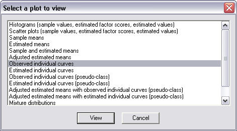
After a plot is selected, a window appears showing ways that the plot can be customized. For example, if observed individual curves are selected, the following window appears:
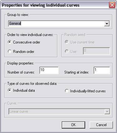
Individual curves can be viewed in consecutive or random order. The window above shows that sets of 10 individual curves will be viewed in consecutive order. Random order can be selected and the number of curves can be changed. The next set of curves are displayed by either selecting the Get next sample item under the Individual data submenu of the Plot menu or by using the arrow button on the toolbar bar.
When viewing a plot, if the mouse is held on a point, information about the variable values for the individual represented by that point are given as shown in the window below.
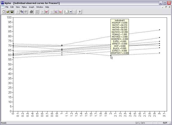
Following is the window that is used to adjust plots of estimated means for different covariate values. A set of covariates is named by typing a name in the edit box next to the Name covariate set button and clicking on the Name covariate set button. The set of covariates for the analysis then appears in the section under Covariate values. The mean or particular values of the covariates can be given for the plot.
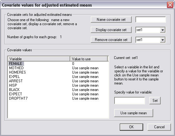
Descriptive statistics can be viewed by using the View descriptive statistics item of the Plot menu which provides the following information for each variable.
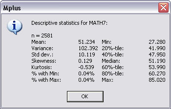
The plots can be exported as a DIB, EMF, or JPEG file using the Export plot to item of the Plot menu. In addition, the data for each plot can be saved in an external file using the Save plot data item of the Plot menu for subsequent use by another program.